Have you ever read a book and found that this book was similar to another book that you had read before? I have already. Practically all self-help books that I read are similar to Napolean Hill’s books.
So I wondered if Natural Language Processing (NLP) could mimic this human ability and find the similarity between documents.
Similarity Problem
To find the similarity between texts you first need to define two aspects:
- The similarity method that will be used to calculate the similarities between the embeddings.
- The algorithm that will be used to transform the text into an embedding, which is a form to represent the text in a vector space.
Similarity Methods
Cosine Similarity
Cosine Similarity measures the cosine of the angle between two embeddings. When the embeddings are pointing in the same direction the angle between them is zero so their cosine similarity is 1 when the embeddings are orthogonal the angle between them is 90 degrees and the cosine similarity is 0 finally when the angle between them is 180 degrees the the cosine similarity is -1.
-1 to 1 is the range of values that the cosine similarity can vary, where the closer to 1 more similar the embeddings are.
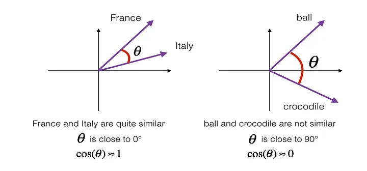
Image from https://datascience-enthusiast.com/DL/Operations_on_word_vectors.html showing a situation where the cosine similarity is 1 because France and Italy are related and other where the similarity is 0 because ball is not similar to crocodile
Mathematically, you can calculate the cosine similarity by taking the dot product between the embeddings and dividing it by the multiplication of the embeddings norms, as you can see in the image below.

Cosine Similarity formula
In python, you can use the cosine_similarity function from the sklearn package to calculate the similarity for you.
Euclidean Distance
Euclidean Distance is probably one of the most known formulas for computing the distance between two points applying the Pythagorean theorem. To get it you just need to subtract the points from the vectors, raise them to squares, add them up and take the square root of them. Did it seem complex? Don’t worry, in the image below it will be easier to understand.
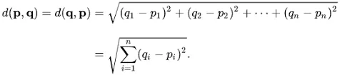
Euclidean Distance formula
In python, you can use the euclidean_distances function also from the sklearn package to calculate it.
There are also other metrics such as Jaccard, Manhattan, and Minkowski distance that you can use, but won’t be discussed in this post.
Are you a talented software developer looking for a long-term remote tech job? Try Index.dev & get matched with high-paid remote jobs with top US, UK, EU companies →
Preprocessing
In NLP problems it is usual to make the text pass first into a preprocessing pipeline. So to all techniques used to transform the text into embeddings, the texts were first preprocessed using the following steps:
- Normalization: transforming the text into lower case and removing all the special characters and punctuations.
- Tokenization: getting the normalized text and splitting it into a list of tokens.
- Removing stop words: stop words are the words that are most commonly used in a language and do not add much meaning to the text. Some examples are the words ‘the’, ‘a’, ‘will’,…
- Stemming: it is the process to get the root of the words and sometimes this root is not equal to the morphological root of the word, but the stemming goal is to make that related word maps to the same stem. Examples: branched and branching become branch.
- Lemmatization: This is the process of getting the same word for a group of inflected word forms, the simplest way to do this is with a dictionary. Examples: is, was, were become be.
The output of this pipeline is a list with the formatted tokens.
Algorithms to transform the text into embeddings
Term Frequency-Inverse Document Frequency (TF-IDF)
Before talking about TF-IDF I am going to talk about the simplest form of transforming the words into embeddings, the Document-term matrix. In this technique you only need to build a matrix where each row is a phrase, each column is a token and the value of the cell is the number of times that a word appeared in the phrase.
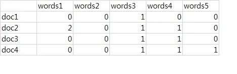
Document-term matrix example
After that to get the similarity between two phrases you only need to choose the similarity method and apply it to the phrases rows. The major problem of this method is that all words are treated as having the same importance in the phrase.
To address this problem TF-IDF emerged as a numeric statistic that is intended to reflect how important a word is to a document.
TF-IDF gets this importance score by getting the term’s frequency (TF) and multiplying it by the term inverse document frequency (IDF). The higher the TF-IDF score the rarer the term in a document and the higher its importance.
How to calculate TF-IDF?
The term frequency it’s how many times a term appears in the document, for example: if the word ‘stock’ appears 20 times in a 2000 words document the TF of stock is 20/2000 = 0.01.
The IDF is logarithmic of the total number of documents divided by the total number of documents that contain the term, for example: if there are 50.000 documents and the word ‘stock’ appears in 500 documents so the IDF is the log(50000/500) = 4.6. So the TF-IDF of ‘stock’ is 4.6 * 0.01 = 0.046.
Word2Vec
In Word2Vec we use neural networks to get the embeddings representation of the words in our corpus (set of documents). The Word2Vec is likely to capture the contextual meaning of the words very well.
To get the word embeddings, you can use two methods: Continuous Bag of Words (CBOW) or Skip Gram. Both of these methods take as input the one-hot encoding representation of the words, to get this representation you just need to build a vector with the size of the number of unique words in your corpus, then each word will be represented as one in a specific position and zeros in all others positions of the vector.
For example, suppose our corpus has only 3 words airplane, bee, and cat. So we can represent them as:
- airplane: [1, 0, 0]
- bee: [0, 1, 0]
- cat: [0, 0, 1]
In Word2Vec we are not interested in the output of the model, but we are interested in the weights of the hidden layer. Those weights will be the embeddings of the words.
CBOW
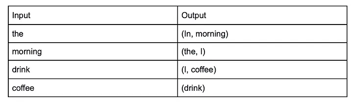
The CBOW model goal is to receive a set of one hot encoding word, predict a word learning the context. So let’s assume that we have the phrase ‘In the morning I drink coffee’, the input and outputs of the CBOW model would be:
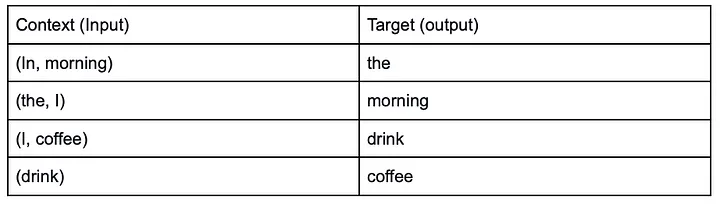
Example of CBOW input and expected output
So it’s a supervised learning model and the neural network learns the weights of the hidden layer using a process called backpropagation.
Skip-Gram
Skip-Gram is like the opposite of CBOW, here a target word is passed as input and the model tries to predict the neighboring words.
Example of Skip-Gram input and expected output
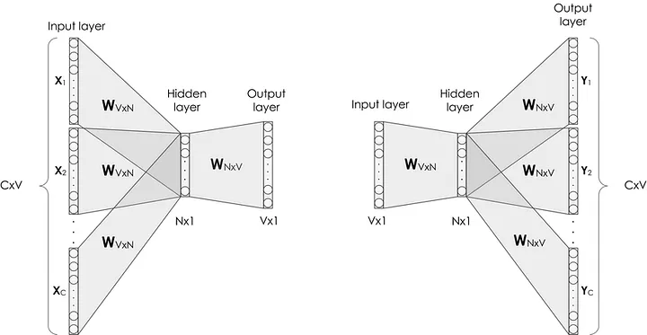
CBOW Architecture in the left and Skip-Gram Architecture in the right
Doc2Vect
In Word2Vec we get one embedding for each one of the words. Word2Vect is useful to do a comparison between words, but what if you want to compare documents?
You could do some vector average of the words in a document to get a vector representation of the document using Word2Vec or you could use a technique built for documents like Doc2Vect.
The Doc2Vect in Gensim is an implementation of the article Distributed Representations of Sentences and Documents by Le and Mikolov. In this article, the authors presented two algorithms to get the embeddings for the documents. The Distributed Memory Model of Paragraph Vectors (PV-DM) and the Distributed Bag of Words version of Paragraph Vector (PV-DBOW)
Distributed Memory Model of Paragraph Vectors (PV-DM)
This model looks like the CBOW, but now the author created a new input to the model called paragraph id.
“The paragraph token can be thought of as another word. It acts as a memory that remembers what is missing from the current context — or the topic of the paragraph.”
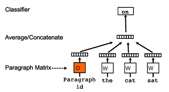
PV-DM Architecture
Distributed Bag of Words version of Paragraph Vector (PV-DBOW)
The PV-DBOW method it is similar to the Skip-Gram, here the input is a paragraph id and the model tries to predict words randomly sampled from the document.
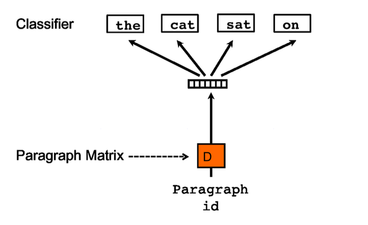
PV-DBOW Architecture
To get a more robust document representation, the author combined the embeddings generated by the PV-DM with the embeddings generated by the PV-DBOW.
Transformers
The Transformers technique is revolutionizing the NLP problems and setting the state-of-art performance with the models BERT and RoBERTa. So in Sentence-BERT: Sentence Embeddings using Siamese BERT-Networks, Reimers and Gurevych modified the model architecture of BERT and RoBERTa to make them output a fixed size sentence embedding.
To achieve that, they added a pooling operation to the output of the transformers, experimenting with some strategies such as computing the mean of all output vectors and computing a max-over-time of the output vectors.
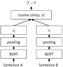
Sentence Embedding BERT to get cosine similarity
To use a pre-trained transformer in python is easy, you just need to use the sentece_transformes package from SBERT. In SBERT is also available multiples architectures trained in different data.
Comparing techniques
The machine used was a MacBook Pro with a 2.6 GHz Dual-Core Intel Core i5 and an 8 GB 1600 MHz DDR3 memory. The data used were the texts from the letters written by Warren Buffet every year to the shareholders of Berkshire Hathaway the company that he is CEO.
The goal was to get the letters that were close to the 2008 letter.
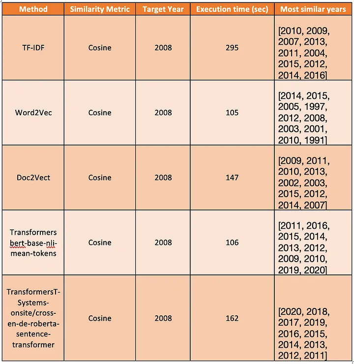
Table with the Method, Similarity Metric, Target Year, Execution time in seconds, and the Most Similar Years ordered by the most similar to the least similar
TF-IDF was the slowest method taking 295 seconds to run since its computational complexity is O(nL log nL), where n is the number of sentences in the corpus and L is the average length of the sentences in a dataset.
One odd aspect was that all the techniques gave different results in the most similar years. Since the data is unlabelled we can not affirm what was the best method. In the next analysis, I will use a labeled dataset to get the answer so stay tuned.
Conclusion
I implemented all the techniques above and you can find the code in this GitHub repository. There you can choose the algorithm to transform the documents into embeddings and you can choose between cosine similarity and Euclidean distances.
The set of texts that I used was the letters that Warren Buffets writes annually to the shareholders from Berkshire Hathaway, the company that he is CEO.
In this article, we have explored the NLP document similarity task. Showing 4 algorithms to transform the text into embeddings: TF-IDF, Word2Vec, Doc2Vect, and Transformers and two methods to get the similarity: cosine similarity and Euclidean distance.
Feel free to reach me with any comments on my Linkedin account and thank you for reading this post.
