Algorithms are the foundation of programming. Each algorithm has a set of instructions or procedures, designed to achieve a specific goal. It can be simple, involving a sequence of basic operations or complex following a multi-step process with different data structures and logic.
No matter how complex algorithms can get, their main goal is to take in input, process it, and provide the answer you need.
What is really crucial for a developer is the capability to think algorithmically. Not just so you can reproduce standard algorithms, but being able to use code and solve whatever problems you may encounter as a programmer.
That’s why we’ve curated a list of 13 Python algorithms that developers should know have in their toolbox, along with code implementation.
Overview of the Algorithms We Cover
There are many ways of classifying algorithms, including implementation method, design method, research area, complexity, and randomness. Examples of algorithms are sorting, searching, graph traversals, string manipulations, and many more.
Here’s a sneak peek of the 13 most important ones we’ll cover:
- Sorting algorithms: These algorithms are essential for organizing data efficiently. We'll look in more detail at quicksort, merge sort, heap sort, and radix sort.
- Search algorithms: They are key for finding elements in large datasets. Examples include binary search and hash tables.
- Graph algorithms: They are used for solving graph-related challenges, like finding the shortest path or checking connectivity. We’ll take a closer look at Breadth-first search, Depth-first search, and Dijkstra’s algorithm.
- Dynamic programming: Think of it as a technique used for breaking down problems into simpler, more manageable chunks to avoid extra work. We’ll deep dive into the Fibonacci Sequence and Bellman-Ford algorithm.
- Greedy algorithms: They are used to solve optimization challenges by making the best choice at each step, even if it doesn't guarantee the absolute best outcome in the long run. A prominent example is Huffman coding.
- Backtracking: They aim to explore all possible combinations, getting rid of paths that don’t lead to an effective solution. We’ll look at the N-Queens problem in detail.
Sorting Algorithms
Quicksort
Quicksort is a divide-and-conquer algorithm that acts as a powered organizer. It picks the “pivot” element from the array and uses it as a dividing line. Then, it whips through the data. Once everything's sorted around the pivot, it dives into those piles and repeats the process until everything is clean.
Code implementation:
def quicksort(arr):
    if len(arr) <= 1:
        return arr
    pivot = arr[len(arr) // 2]
    left = [x for x in arr if x < pivot]
    middle = [x for x in arr if x == pivot]
    right = [x for x in arr if x > pivot]
    return quicksort(left) + middle + quicksort(right)

# Example usage:
arr = [3, 6, 8, 10, 1, 2, 1]
sorted_arr = quicksort(arr)
print(sorted_arr)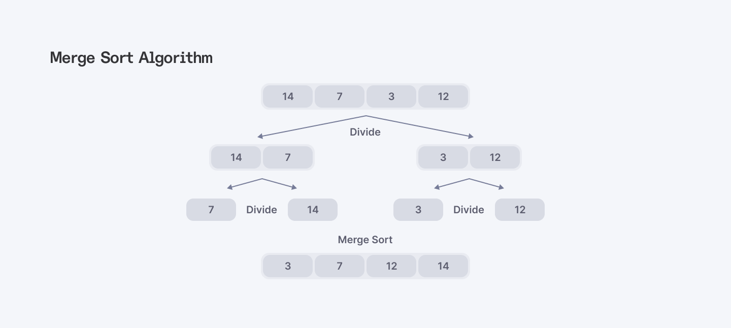
Merge Sort
This algorithm is a divide and conquer master. It splits the array in half, sorts each half individually, and then merges those sorted halves back together into an ordered collection.
Code implementation:
def merge_sort(arr):
    if len(arr) <= 1:
        return arr

    # Divide the array into two halves
    mid = len(arr) // 2
    left_half = arr[:mid]
    right_half = arr[mid:]

    # Recursively sort each half
    left_half = merge_sort(left_half)
    right_half = merge_sort(right_half)

    # Merge the sorted halves
    return merge(left_half, right_half)

def merge(left, right):
    result = []
    left_idx = 0
    right_idx = 0

    # Merge two sorted arrays
    while left_idx < len(left) and right_idx < len(right):
        if left[left_idx] <= right[right_idx]:
            result.append(left[left_idx])
            left_idx += 1
        else:
            result.append(right[right_idx])
            right_idx += 1

    # Append remaining elements
    result.extend(left[left_idx:])
    result.extend(right[right_idx:])

    return result

# Example usage:
arr = [3, 6, 8, 10, 1, 2, 1]
sorted_arr = merge_sort(arr)
print(sorted_arr)
Heap Sort
This one is a little different. Heap sort is a comparison-based sorting algorithm that relies on a binary heap data structure. It transforms the input array into a maximum heap, repeatedly removes the largest element, and places it at the end until the array is sorted.
Code implementation:
def heapify(arr, n, i):
    largest = i  # Initialize largest as root
    left = 2 * i + 1  # Left child position
    right = 2 * i + 2  # Right child position

    # Check if left child exists and is greater than root
    if left < n and arr[left] > arr[largest]:
        largest = left

    # Check if right child exists and is greater than root
    if right < n and arr[right] > arr[largest]:
        largest = right

    # Change root if needed
    if largest != i:
        arr[i], arr[largest] = arr[largest], arr[i]  # Swap

        # Heapify the root.
        heapify(arr, n, largest)

def heap_sort(arr):
    n = len(arr)

    # Build a maxheap.
    for i in range(n // 2 - 1, -1, -1):
        heapify(arr, n, i)

    # Extract elements one by one
    for i in range(n - 1, 0, -1):
        arr[i], arr[0] = arr[0], arr[i]  # Swap
        heapify(arr, i, 0)

# Example usage:
arr = [3, 6, 8, 10, 1, 2, 1]
heap_sort(arr)
print("Sorted array:", arr)
Radix Sort
Radix sort is a non-comparison sorting algorithm. It organizes an array by sorting the digits of the elements, starting from the least significant digit to the most significant one. Radix Sort is fast, but not stable. Plus, it’s not as efficient as Merge Sort for large arrays with many unique elements.
Code implementation:
def counting_sort(arr, exp):
    n = len(arr)
    output = [0] * n
    count = [0] * 10

    # Store count of occurrences in count[]
    for i in range(n):
        index = (arr[i] // exp) % 10
        count[index] += 1

    # Change count[i] so that count[i] contains the actual position of this digit in output[]
    for i in range(1, 10):
        count[i] += count[i - 1]

    # Build the output array
    i = n - 1
    while i >= 0:
        index = (arr[i] // exp) % 10
        output[count[index] - 1] = arr[i]
        count[index] -= 1
        i -= 1

    # Copy the output array to arr[], so that arr now contains sorted numbers according to current digit
    for i in range(len(arr)):
        arr[i] = output[i]

def radix_sort(arr):
    # Find the maximum number to know the number of digits
    max_num = max(arr)

    # Do counting sort for every digit. Note that instead of passing the digit number, exp is passed. exp is 10^i where i is the current digit number
    exp = 1
    while max_num // exp > 0:
        counting_sort(arr, exp)
        exp *= 10

# Example usage:
arr = [170, 45, 75, 90, 802, 24, 2, 66]
radix_sort(arr)
print("Sorted array:", arr)
Search Algorithms
Binary Search
Binary search is a divide-and-conquer algorithm that finds an item in a sorted array by repeatedly dividing it in half, discarding half it knows the item isn’t in, until the target value is found.
Code implementation:
def binary_search(arr, target):
    low = 0
    high = len(arr) - 1

    while low <= high:
        mid = (low + high) // 2  # Calculate mid point

        # Check if target is present at mid
        if arr[mid] == target:
            return mid

        # If target is greater, ignore left half
        elif arr[mid] < target:
            low = mid + 1

        # If target is smaller, ignore right half
        else:
            high = mid - 1

    # Target is not present in array
    return -1

# Example usage:
arr = [1, 3, 5, 7, 9, 11, 13, 15]
target = 7
result = binary_search(arr, target)

if result != -1:
    print(f"Element {target} is present at index {result}.")
else:
    print(f"Element {target} is not present in the array.")
Hash Tables
A hash table is a data structure that stores key-value pairs. By using a hash function, it calculates an index where the value is stored in an array. This allows quick access to the value based on its key, making storing and retrieving data more efficient.
Code implementation:
class HashTable:
    def __init__(self, size):
        self.size = size
        self.table = [[] for _ in range(size)]

    def _hash_function(self, key):
        return hash(key) % self.size

    def insert(self, key, value):
        index = self._hash_function(key)
        for pair in self.table[index]:
            if pair[0] == key:
                pair[1] = value
                return
        self.table[index].append([key, value])

    def get(self, key):
        index = self._hash_function(key)
        for pair in self.table[index]:
            if pair[0] == key:
                return pair[1]
        raise KeyError(f'Key {key} not found')

    def delete(self, key):
        index = self._hash_function(key)
        for i, pair in enumerate(self.table[index]):
            if pair[0] == key:
                del self.table[index][i]
                return
        raise KeyError(f'Key {key} not found')

# Example usage:
hash_table = HashTable(10)
hash_table.insert('apple', 5)
hash_table.insert('banana', 7)
hash_table.insert('cherry', 10)

print(hash_table.get('banana'))  # Output: 7

hash_table.delete('banana')
print(hash_table.get('banana'))  # Raises KeyError: 'Key banana not found'
Graph Algorithms
Breadth-First Search (BFS)
Breadth-First Search (BFS) is a graph traversal algorithm that explores all nodes at the current depth level before moving to the next level. BFS starts at a source node, visits all its neighbors, then moves to their neighbors, continuing until all nodes are visited or the target is found. Finding the shortest path between two nodes and detecting graph cycles are its best uses.
Code implementation:
from collections import deque

def bfs(graph, start):
    # Initialize a queue for BFS and add the start node
    queue = deque([start])
    # Set to keep track of visited nodes
    visited = set()
    # Mark the start node as visited
    visited.add(start)

    while queue:
        # Dequeue a node from the queue
        node = queue.popleft()
        print(node, end=" ")

        # Get all adjacent nodes of the dequeued node
        for neighbor in graph[node]:
            if neighbor not in visited:
                # If a neighbor has not been visited, mark it as visited and enqueue it
                visited.add(neighbor)
                queue.append(neighbor)

# Example graph as an adjacency list
graph = {
    'A': ['B', 'C'],
    'B': ['D', 'E'],
    'C': ['F'],
    'D': [],
    'E': ['F'],
    'F': []
}

# Perform BFS starting from node 'A'
bfs(graph, 'A')
Depth-First Search (DFS)
Depth-First Search (DFS) is a graph traversal algorithm that explores a graph by following one path to its end, then backtracking and trying other paths. Finding all paths between two nodes and detecting strongly connected components in a graph are among its best uses.
Recursive DFS Code Implementation:
def dfs_recursive(graph, node, visited=None):
    if visited is None:
        visited = set()
    visited.add(node)
    print(node, end=" ")

    for neighbor in graph[node]:
        if neighbor not in visited:
            dfs_recursive(graph, neighbor, visited)

# Example graph as an adjacency list
graph = {
    'A': ['B', 'C'],
    'B': ['D', 'E'],
    'C': ['F'],
    'D': [],
    'E': ['F'],
    'F': []
}

# Perform DFS starting from node 'A'
dfs_recursive(graph, 'A')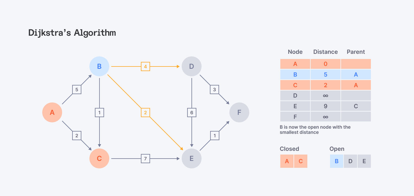
Dijkstra’s Algorithm
Dijkstra’s algorithm is used to find the shortest path between a single source node and all other nodes in a graph. While it doesn't always select the best path at each step, it guarantees the shortest path to each node in the end.
Code implementation:
import heapq
from collections import defaultdict, deque

def dijkstra(graph, start):
    # Initialize distances from the start node to all other nodes as infinity
    distances = {node: float('inf') for node in graph}
    distances[start] = 0

    # Priority queue to store nodes to be explored, starting with the start node
    pq = [(0, start)]  # (distance, node)

    while pq:
        current_distance, current_node = heapq.heappop(pq)

        # If current distance is greater than known distance, skip
        if current_distance > distances[current_node]:
            continue

        # Visit each neighbor of the current node
        for neighbor, weight in graph[current_node].items():
            distance = current_distance + weight

            # If a shorter path to neighbor is found, update distance and push to priority queue
            if distance < distances[neighbor]:
                distances[neighbor] = distance
                heapq.heappush(pq, (distance, neighbor))

    return distances

# Example graph as an adjacency list with weights
graph = {
    'A': {'B': 6, 'D': 1},
    'B': {'A': 6, 'C': 5, 'D': 2, 'E': 2},
    'C': {'B': 5, 'E': 5},
    'D': {'A': 1, 'B': 2, 'E': 1},
    'E': {'B': 2, 'C': 5, 'D': 1}
}

# Perform Dijkstra's algorithm starting from node 'A'
start_node = 'A'
shortest_distances = dijkstra(graph, start_node)

# Print shortest distances from the start node to all other nodes
for node, distance in shortest_distances.items():
    print(f"Shortest distance from {start_node} to {node} is {distance}")
Ready for a high-paying remote Python career? Join Index.dev and connect with top companies in the UK, EU, and US. Register now!
Dynamic Programming
Fibonacci Sequence
The Fibonacci sequence defines a function that calculates each Fibonacci number as the sum of the two preceding ones, starting with 0 and 1. This is done through using recursion or iteration, building the sequence step by step from these initial values.
Code implementation:
def fibonacci_recursive(n):
    if n <= 0:
        return 0
    elif n == 1:
        return 1
    else:
        return fibonacci_recursive(n-1) + fibonacci_recursive(n-2)

# Example usage:
print(fibonacci_recursive(10))
Bellman-Ford Algorithm
The Bellman-Ford algorithm calculates the shortest paths from a single source node to all other nodes in a graph. It’s similar to Dijkstra’s algorithm, but it can handle negative edge weights. This makes it suitable for graphs where some edges have negative weights.
Code implementation:
class Graph:
    def __init__(self, vertices):
        self.vertices = vertices
        self.edges = []

    def add_edge(self, u, v, weight):
        self.edges.append([u, v, weight])

    def bellman_ford(self, source):
        distance = [float('inf')] * self.vertices
        distance[source] = 0

        for _ in range(self.vertices - 1):
            for u, v, weight in self.edges:
                if distance[u] != float('inf') and distance[u] + weight < distance[v]:
                    distance[v] = distance[u] + weight

        for u, v, weight in self.edges:
            if distance[u] != float('inf') and distance[u] + weight < distance[v]:
                print("Graph contains negative weight cycle")
                return

        self.print_solution(distance)

    def print_solution(self, distance):
        print("Vertex Distance from Source")
        for i in range(self.vertices):
            print(f"{i}\t\t{distance[i]}")

# Example usage:
g = Graph(5)
g.add_edge(0, 1, -1)
g.add_edge(0, 2, 4)
g.add_edge(1, 2, 3)
g.add_edge(1, 3, 2)
g.add_edge(1, 4, 2)
g.add_edge(3, 2, 5)
g.add_edge(3, 1, 1)
g.add_edge(4, 3, -3)

g.bellman_ford(0)
Greedy Algorithms
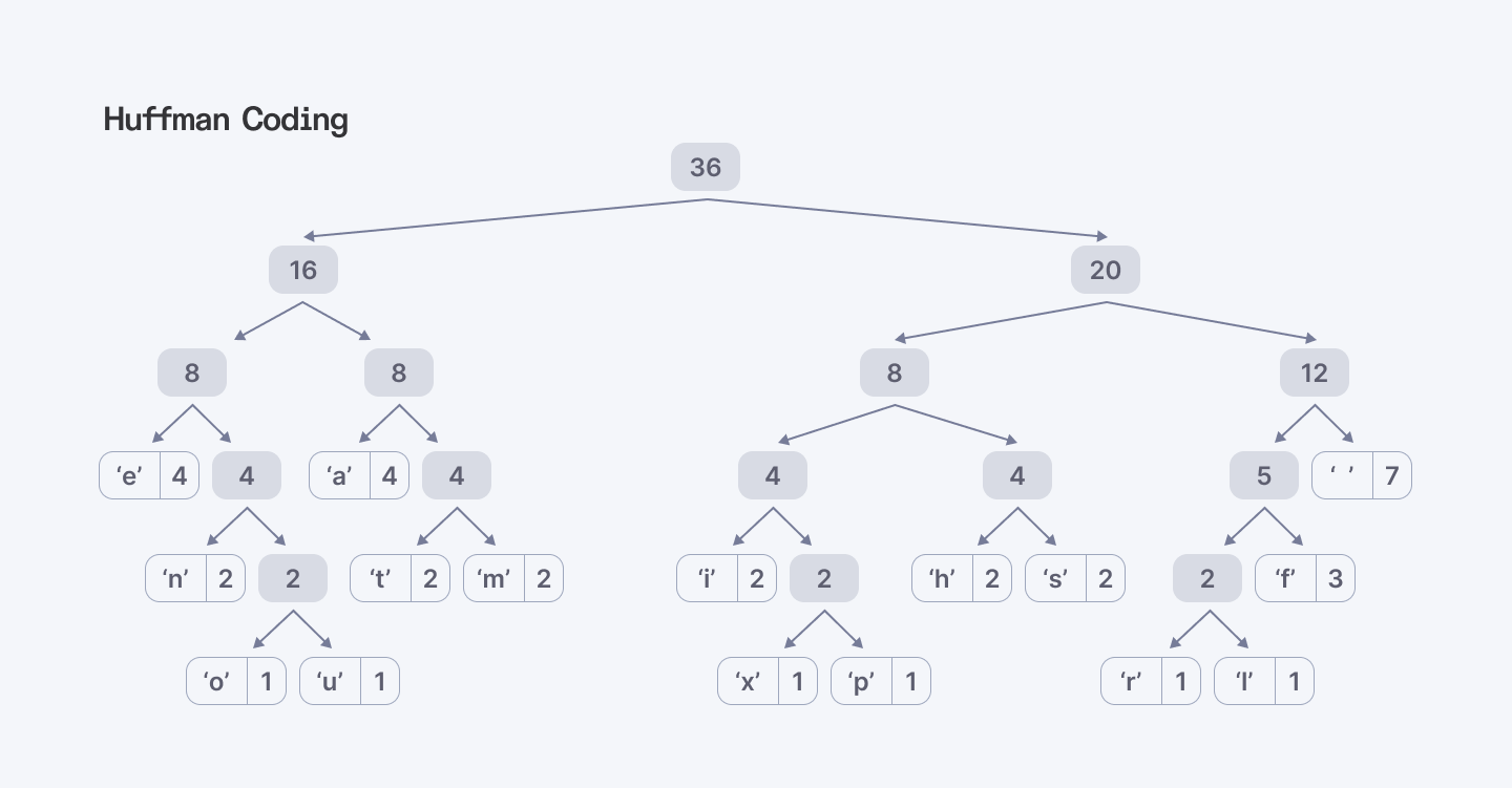
Huffman Coding
Huffman coding is a lossless data compression technique that uses a greedy algorithm to create prefix codes for a set of symbols. It analyzes character frequency and arranges them in a tree, where more frequent characters have shorter codes and less frequent characters have longer codes. This significantly reduces the overall data size, making it a fundamental method for text compression.
Code implementation:
import heapq
from collections import defaultdict, Counter

class Node:
    def __init__(self, char=None, freq=None):
        self.char = char
        self.freq = freq
        self.left = None
        self.right = None

    # Define comparators for priority queue
    def __lt__(self, other):
        return self.freq < other.freq

def build_huffman_tree(text):
    # Count frequency of each character
    frequency = Counter(text)

    # Create a priority queue with initial nodes
    priority_queue = [Node(char, freq) for char, freq in frequency.items()]
    heapq.heapify(priority_queue)

    # Iterate until only one node is left (the root)
    while len(priority_queue) > 1:
        left = heapq.heappop(priority_queue)
        right = heapq.heappop(priority_queue)
        merged = Node(freq=left.freq + right.freq)
        merged.left = left
        merged.right = right
        heapq.heappush(priority_queue, merged)

    return priority_queue[0]

def build_codes(node, prefix="", codebook={}):
    if node is not None:
        if node.char is not None:
            codebook[node.char] = prefix
        build_codes(node.left, prefix + "0", codebook)
        build_codes(node.right, prefix + "1", codebook)
    return codebook

def huffman_encoding(text):
    root = build_huffman_tree(text)
    huffman_codebook = build_codes(root)
    encoded_text = "".join(huffman_codebook[char] for char in text)
    return encoded_text, huffman_codebook

def huffman_decoding(encoded_text, codebook):
    reverse_codebook = {v: k for k, v in codebook.items()}
    current_code = ""
    decoded_text = []

    for bit in encoded_text:
        current_code += bit
        if current_code in reverse_codebook:
            decoded_text.append(reverse_codebook[current_code])
            current_code = ""

    return "".join(decoded_text)

# Example usage
text = "this is an example for huffman encoding"
encoded_text, codebook = huffman_encoding(text)
print(f"Encoded Text: {encoded_text}")
print(f"Codebook: {codebook}")

decoded_text = huffman_decoding(encoded_text, codebook)
print(f"Decoded Text: {decoded_text}")
Backtracking Algorithms
The N-Queens Problem
The N-Queens problem can be solved using backtracking. It involves placing N queens on an NxN chessboard so that no two queens threaten each other. The algorithm aims to place queens row by row, ensuring each queen’s position is safe from attacks from previous queens. If a conflict arises, it backtracks and explores alternative placements until a solution is found.
def is_safe(board, row, col):
    # Check if there's a queen in the same column
    for i in range(row):
        if board[i][col] == 1:
            return False

    # Check upper left diagonal
    for i, j in zip(range(row, -1, -1), range(col, -1, -1)):
        if board[i][j] == 1:
            return False

    # Check upper right diagonal
    for i, j in zip(range(row, -1, -1), range(col, len(board))):
        if board[i][j] == 1:
            return False

    return True

def solve_n_queens_util(board, row):
    n = len(board)
    # Base case: If all queens are placed, return True
    if row >= n:
        return True

    for col in range(n):
        # Check if the queen can be placed in board[row][col]
        if is_safe(board, row, col):
            # Place the queen
            board[row][col] = 1

            # Recur to place rest of the queens
            if solve_n_queens_util(board, row + 1):
                return True

            # If placing queen in board[row][col] doesn't lead to a solution, backtrack
            board[row][col] = 0

    # If no position is found to place the queen in this row, return False
    return False

def solve_n_queens(n):
    # Initialize the board
    board = [[0] * n for _ in range(n)]

    # Start solving from the first row
    if not solve_n_queens_util(board, 0):
        print(f"No solution exists for {n}-Queens problem.")
        return

    # Print the board
    for row in board:
        print(row)

# Example usage:
n = 4
solve_n_queens(n)
Wrapping Up
Software engineering is about being able to challenge problems and build solutions. Learning algorithms is key because they teach you how to approach problems and always find a better way to solve it. These algorithms are used in a wide range of applications, from web development to machine learning. Knowing how to implement can significantly make you become a better developer and more efficient problem-solver.
Ready to build amazing things with Python? Join Index.dev's developer network and access high-paying, long-term remote projects.
Got a project? Let’s talk! Index.dev can assist you in selecting and hiring highly-skilled Python developers who understand how to manage data structures and functions in the construction of high-performance applications.
Index developers can help you:
- Use the best performing algorithms and data structures of processing.
- Take advantage of Python and its attributes and libraries for efficient data manipulation.
- Use clean, readable, and scalable code in order to solve any challenge.
With a vast database of resources and stringent vetting techniques, you get Python specialists with good command of data manipulation, data structures, and functions.
