How to Generate Realistic Data for Machine Learning using Python

Realistic data generation isn’t optional anymore—it’s a core skill for machine learning and data science. As models become more advanced, the ability to generate high-quality synthetic data gives you a serious edge. It helps you test and refine models when real-world data is limited, biased, or just too sensitive to use directly.

If you need to create fake user profiles, Faker has you covered. Simulating sensor data? NumPy and Pandas can handle it. Working with time-series or correlated data? There are solid techniques for that too.

I’ll walk you through practical, production-ready methods for generating synthetic data that mirrors real-world complexity. By the end, you’ll have tools you can plug directly into your ML pipelines to make sure your models are battle-tested. Let’s get started.

Join Index.dev to work remotely on top AI and machine learning projects with global companies. Apply today!

Concept Explanation

Effective data simulation goes far beyond generating random numbers. The goal is to capture the statistical properties of real-world data: variability, trends, distributions, inter-variable correlations, and noise patterns.

• Realistic Distributions: Using libraries like NumPy and Pandas, we can simulate natural variability (e.g., Gaussian noise for sensor data) and introduce controlled randomness that reflects actual operational conditions.
• Complex Patterns: Our examples include seasonal trends with multiple frequency components and deliberate anomalies. This approach allows you to mimic behaviors seen in domains like finance or IoT, where unexpected events can drastically impact model performance.
• Modular and Reusable Code: We encapsulate the simulation logic into functions and classes. For example, our class-based sensor and time-series simulators are designed with configurable parameters, enabling you to adapt the code easily for different scenarios.
• Direct Application to ML Pipelines: The code converts simulation outputs into Pandas DataFrames, which are directly usable in machine learning frameworks such as scikit-learn or TensorFlow. Each example is tailored to show not just how to generate data, but why each component - be it trend, seasonality, or noise - is essential for realistic simulation.

Why This Matters

In machine learning, your model is only as good as the data it learns from. Traditional approaches often fall short:

• Randomly generated data lacks the subtle patterns of real-world systems
• Static datasets can't capture the dynamic nature of evolving environments
• Overly simplistic simulations lead to models that fail in production

Our techniques address these challenges by providing:

• Statistically sound data generation
• Flexibility to model complex domain-specific behaviors
• Easy integration with existing machine learning workflows

Learn More: AI vs Machine Learning vs Data Science: What Should You Learn in 2025?

The Approach

1. Simulating User Data with Faker

When developing and testing applications that handle user data, we often need realistic sample data that mimics actual user information. This becomes crucial during development phases where we want to maintain data privacy while still working with believable user profiles. Let's explore how we can generate such data efficiently using the Faker library.

from faker import Faker
import pandas as pd
from datetime import datetime

fake = Faker()

def generate_enhanced_user_data(n, include_demographics=True):
    """
    Generate realistic user profiles with optional demographic information
    
    Args:
        n (int): Number of user profiles to generate
        include_demographics (bool): Whether to include additional demographic data
        
    Returns:
        pd.DataFrame: DataFrame containing generated user profiles
    """
    data = []
    for _ in range(n):
        profile = fake.simple_profile()
        user_data = {
            "user_id": fake.uuid4(),
            "name": profile['name'],
            "sex": profile['sex'],
            "address": profile['address'],
            "email": profile['mail'],
            "birthdate": profile['birthdate'],
            "registration_date": fake.date_between(
                start_date='-2y', 
                end_date='today'
            )
        }
        
        if include_demographics:
            user_data.update({
                "occupation": fake.job(),
                "income_bracket": fake.random_element(
                    elements=('Low', 'Medium', 'High')
                ),
                "education_level": fake.random_element(
                    elements=('High School', 'Bachelor', 'Master', 'PhD')
                )
            })
        
        data.append(user_data)
    
    df = pd.DataFrame(data)
    df['age'] = (datetime.now().year - 
                 pd.to_datetime(df['birthdate']).dt.year)
    
    return df

# Generate enhanced user profiles
df_users = generate_enhanced_user_data(10, include_demographics=True)

Explanation:

• Why Faker? We use the Faker library to simulate realistic user profiles. Faker provides a simple API to generate fake yet plausible data, which is especially useful for testing and prototyping.
• Why a Function with Parameters? We use a flexible function structure with configurable parameters to make the code reusable across different scenarios. The include_demographics parameter lets us optionally generate additional user information based on our needs.
• UUID and Registration Date: Each user gets a unique identifier and registration date to mimic real database records. This is crucial for testing database operations and user analytics.
• Data Enrichment: The enhanced profile includes calculated fields like age and optional demographic data. This helps in testing data aggregation and filtering operations common in real applications.
• DataFrame Advantages: Converting to a Pandas DataFrame gives us immediate access to powerful data manipulation tools. The automatic age calculation using pandas datetime operations shows how we can derive new insights from existing fields.

2. Advanced Sensor Data Simulation using NumPy and Pandas

In IoT and industrial applications, we often need to simulate sensor data for testing and development purposes. This implementation creates realistic sensor readings with configurable parameters and built-in anomaly detection capabilities.

import numpy as np
import pandas as pd
from typing import Dict, Optional

class SensorDataSimulator:
    def __init__(
        self,
        base_temperature: float = 25.0,
        temp_variance: float = 2.0,
        humidity_range: Dict[str, float] = {"min": 30.0, "max": 70.0},
        anomaly_rate: float = 0.02
    ):
        """
        Initialize the sensor simulator with configurable parameters
        """
        self.base_temperature = base_temperature
        self.temp_variance = temp_variance
        self.humidity_range = humidity_range
        self.anomaly_rate = anomaly_rate
        
    def generate_readings(
        self,
        n_readings: int,
        start_date: Optional[str] = None,
        frequency: str = "1min"
    ) -> pd.DataFrame:
        """
        Generate sensor readings with optional anomalies
        """
        if start_date is None:
            start_date = pd.Timestamp.now().strftime("%Y-%m-%d")
            
        timestamps = pd.date_range(
            start_date,
            periods=n_readings,
            freq=frequency
        )
        
        # Generate base temperature readings
        temperature = np.random.normal(
            loc=self.base_temperature,
            scale=self.temp_variance,
            size=n_readings
        )
        
        # Add daily temperature variation (peak at noon)
        hour_of_day = timestamps.hour + timestamps.minute / 60.0
        daily_variation = 2 * np.sin(2 * np.pi * (hour_of_day - 6) / 24)
        temperature += daily_variation
        
        # Generate humidity with daily patterns
        humidity_base = np.random.uniform(
            self.humidity_range["min"],
            self.humidity_range["max"],
            size=n_readings
        )
        humidity = humidity_base - daily_variation  # Inverse relationship
        
        # Add anomalies
        anomaly_mask = np.random.random(n_readings) < self.anomaly_rate
        temperature[anomaly_mask] += np.random.normal(
            0, self.temp_variance * 3, sum(anomaly_mask)
        )
        
        return pd.DataFrame({
            "timestamp": timestamps,
            "temperature": temperature,
            "humidity": humidity,
            "is_anomaly": anomaly_mask
        })

# Initialize and use the simulator
sensor_sim = SensorDataSimulator()
df_sensor = sensor_sim.generate_readings(
    n_readings=1440,  # One day of minute-by-minute readings
    frequency="1min"
)

Explanation:

• Why Class-Based Design? Using a class structure helps encapsulate all related functionality and configuration. This makes the code more maintainable and allows for multiple simulator instances with different settings.
• Daily Variations: We incorporate sine waves for temperature variations to mimic real-world patterns. The inverse relationship between temperature and humidity reflects natural environmental behaviors.
• Anomaly Generation: Random anomalies are intentionally injected to help test monitoring systems. The anomaly rate is configurable, making it useful for different testing scenarios.
• Timestamp Handling: Using pandas' date_range with configurable frequency allows for flexible time series generation. This is essential when testing different data collection intervals.
• Statistical Simulation: Temperature data is modeled using a normal distribution (via np.random.normal), reflecting natural variability around a mean value, while humidity is simulated using a uniform distribution to cover a broader range.
• DataFrame Assembly: The simulated data is then encapsulated in a DataFrame, which is the standard structure for data analysis in Python.

3. Generating Synthetic Regression Data 

When developing machine learning models, having controllable regression datasets helps in understanding model behavior under different conditions. Let's create a sophisticated regression data generator that can produce datasets with specific characteristics.

import numpy as np
from sklearn.datasets import make_regression
from dataclasses import dataclass
import pandas as pd

@dataclass
class RegressionDataConfig:
    n_samples: int = 100
    n_features: int = 1
    noise: float = 10.0
    bias: float = 0.0
    random_state: int = 42

class RegressionDataGenerator:
    def __init__(self, config: RegressionDataConfig):
        self.config = config
    
    def generate_data(self, add_nonlinearity=False):
        X, y = make_regression(
            n_samples=self.config.n_samples,
            n_features=self.config.n_features,
            noise=self.config.noise,
            bias=self.config.bias,
            random_state=self.config.random_state
        )
        
        if add_nonlinearity:
            # Add polynomial terms
            y = y + 0.3 * np.power(X, 2).sum(axis=1)
        
        # Convert to DataFrame with meaningful column names
        feature_cols = [f'feature_{i+1}' for i in range(self.config.n_features)]
        df = pd.DataFrame(X, columns=feature_cols)
        df['target'] = y
        
        return df

# Generate both linear and nonlinear datasets
config = RegressionDataConfig(n_samples=150, noise=15)
generator = RegressionDataGenerator(config)

linear_data = generator.generate_data()
nonlinear_data = generator.generate_data(add_nonlinearity=True)

Explanation:

• Why DataClass? Using a dataclass for configuration makes it easy to specify and modify data generation parameters. This is especially useful when experimenting with different dataset characteristics.
• Class Structure: The generator class separates configuration from generation logic. This makes the code more organized and allows for easy addition of new generation features.
• Nonlinearity Option: We include an option to add polynomial terms to create nonlinear relationships. This helps in testing how models handle different types of relationships in the data.
• DataFrame Output: Converting to a DataFrame with meaningful column names makes the data immediately usable in analysis workflows. This matches real-world data science practices.

4. Simulating Seasonal Time-Series Data with Anomalies

Time-series data is critical in many domains, from financial forecasting to environmental monitoring. We'll create a robust simulator that generates realistic time-series data with seasonal patterns, trends, and unexpected anomalies.

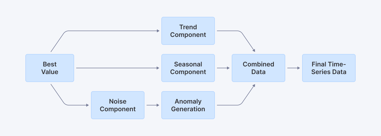
This diagram illustrates how a seasonal time-series simulation integrates a base value, trend, seasonal patterns, noise, and anomalies into the final data.

import numpy as np
import pandas as pd
import matplotlib.pyplot as plt
from typing import Optional, Tuple

class SeasonalTimeSeriesSimulator:
    def __init__(
        self, 
        base_value: float = 0, 
        trend_slope: float = 0.1,
        seasonal_amplitude: float = 5,
        noise_scale: float = 1.5,
        anomaly_config: Optional[Dict[str, float]] = None
    ):
        """
        Initialize seasonal time series simulator with configurable parameters
        """
        self.base_value = base_value
        self.trend_slope = trend_slope
        self.seasonal_amplitude = seasonal_amplitude
        self.noise_scale = noise_scale
        
        # Default anomaly configuration
        self.anomaly_config = anomaly_config or {
            'probability': 0.05,
            'magnitude': 20,
            'variability': 5
        }
    
    def generate_series(
        self, 
        days: int = 365, 
        start_date: Optional[str] = None
    ) -> pd.DataFrame:
        """
        Generate a seasonal time series with trend, seasonality, and anomalies
        """
        # Establish date range
        start_date = start_date or '2023-01-01'
        dates = pd.date_range(start=start_date, periods=days, freq='D')
        
        # Generate trend component
        trend = np.linspace(0, self.trend_slope * days, days)
        
        # Create seasonal component using multiple frequency components
        day_of_year = np.arange(days)
        seasonal = (
            self.seasonal_amplitude * np.sin(2 * np.pi * day_of_year / 365) +
            0.5 * self.seasonal_amplitude * np.sin(2 * np.pi * day_of_year / 30)  # Monthly variation
        )
        
        # Generate noise
        noise = np.random.normal(
            loc=0, 
            scale=self.noise_scale, 
            size=days
        )
        
        # Combine base components
        data = self.base_value + trend + seasonal + noise
        
        # Anomaly generation
        anomalies = self._generate_anomalies(days)
        data_with_anomalies = data + anomalies
        
        # Create DataFrame
        df = pd.DataFrame({
            'date': dates,
            'value': data_with_anomalies,
            'is_anomaly': anomalies != 0
        })
        
        return df
    
    def _generate_anomalies(self, days: int) -> np.ndarray:
        """
        Generate random anomalies based on configuration
        """
        config = self.anomaly_config
        anomalies = np.random.choice(
            [0, 1], 
            size=days, 
            p=[1 - config['probability'], config['probability']]
        )
        
        anomaly_effect = anomalies * np.random.normal(
            loc=config['magnitude'], 
            scale=config['variability'], 
            size=days
        )
        
        return anomaly_effect

# Simulate and visualize
simulator = SeasonalTimeSeriesSimulator()
df_seasonal = simulator.generate_series(days=365)

plt.figure(figsize=(12, 6))
plt.plot(df_seasonal['date'], df_seasonal['value'], label='Simulated Value')
plt.scatter(
    df_seasonal[df_seasonal['is_anomaly']]['date'], 
    df_seasonal[df_seasonal['is_anomaly']]['value'], 
    color='red', 
    label='Anomalies'
)
plt.title("Advanced Seasonal Time-Series Data with Anomalies")
plt.xlabel("Date")
plt.ylabel("Value")
plt.legend()
plt.show()

Explanation:

• Why Class-Based Design? The object-oriented approach allows for highly configurable time series generation. We can easily modify base parameters like trend, seasonality, and noise characteristics to help mimic real-life fluctuations.
• Multiple Frequency Components: By combining sine waves with different periods, we create more realistic seasonal patterns that mimic complex real-world time series data.
• Anomaly Sophistication: The anomaly generation is configurable, allowing precise control over probability, magnitude, and variability of unexpected events.
• Visualization Enhancement: We added anomaly highlighting to make it easier to understand where unexpected events occur in the time series.

5. Generating Multi-Dimensional Correlated Data

In many machine learning and statistical modeling scenarios, understanding the relationships between variables is crucial. We'll create a sophisticated simulator that generates multi-dimensional data with specified correlations.

import numpy as np
import pandas as pd
import seaborn as sns
import matplotlib.pyplot as plt
from typing import List, Union

class MultiVariateDataGenerator:
    def __init__(
        self, 
        feature_means: List[float],
        feature_std: Union[List[float], float] = 1.0,
        correlation_matrix: Optional[np.ndarray] = None
    ):
        """
        Initialize multivariate data generator
        
        Args:
            feature_means: Mean values for each feature
            feature_std: Standard deviation for each feature
            correlation_matrix: Custom correlation matrix
        """
        self.feature_means = feature_means
        
        # Handle standard deviation inputs
        if isinstance(feature_std, (int, float)):
            self.feature_std = [feature_std] * len(feature_means)
        else:
            self.feature_std = feature_std
        
        # Generate correlation matrix if not provided
        if correlation_matrix is None:
            self.correlation_matrix = self._generate_random_correlation(len(feature_means))
        else:
            self.correlation_matrix = correlation_matrix
    
    def _generate_random_correlation(self, n_features: int) -> np.ndarray:
        """
        Generate a random positive semi-definite correlation matrix
        """
        # Create a random matrix and convert to correlation matrix
        random_matrix = np.random.rand(n_features, n_features)
        correlation = np.corrcoef(random_matrix)
        return np.abs(correlation)
    
    def generate_data(self, n_samples: int = 500) -> pd.DataFrame:
        """
        Generate correlated multivariate data
        """
        # Compute covariance matrix
        cov_matrix = np.diag(self.feature_std) @ self.correlation_matrix @ np.diag(self.feature_std)
        
        # Generate multivariate normal data
        data = np.random.multivariate_normal(
            mean=self.feature_means,
            cov=cov_matrix,
            size=n_samples
        )
        
        # Convert to DataFrame
        feature_names = [f'Feature_{i+1}' for i in range(len(self.feature_means))]
        df = pd.DataFrame(data, columns=feature_names)
        
        return df
    
    def visualize_correlations(self, df: pd.DataFrame):
        """
        Create a comprehensive visualization of data correlations
        """
        plt.figure(figsize=(10, 8))
        sns.heatmap(
            df.corr(), 
            annot=True, 
            cmap='coolwarm', 
            linewidths=0.5
        )
        plt.title("Feature Correlation Heatmap")
        plt.tight_layout()
        plt.show()

# Usage example
generator = MultiVariateDataGenerator(
    feature_means=[50, 30, 20],
    feature_std=[5, 3, 2]
)
df_correlated = generator.generate_data(n_samples=1000)
generator.visualize_correlations(df_correlated)

Explanation:

• Why Flexible Initialization? The generator supports various input types for means, standard deviations, and correlation matrices, making it adaptable to different data generation scenarios.
• Correlation Matrix Generation: We include a method to generate random correlation matrices, allowing for automatic correlation structure when not explicitly specified.
• Advanced Visualization: The correlation heatmap provides an immediate visual understanding of the relationships between generated features.
• Realistic Data Simulation: By using multivariate normal distribution with controlled parameters, we can create datasets that mimic real-world complex relationships between variables.

Explore More: Understanding Data Types in Python Programming

Best Practices

Validate with Visualization

Always plot your simulated data using Matplotlib or Seaborn to confirm that it mirrors expected real-world behavior. For instance, the scatter matrix and heatmap visualizations in our multi-dimensional and correlation examples help verify feature relationships.

Use Parameterized Functions and Classes

Modular design (using functions and classes) enhances code reusability and maintainability. Our approach uses parameterized constructors and configurable functions so that you can easily adapt simulations to varying requirements.

Incorporate Controlled Randomness

Balance randomness with control. Use distributions (like Gaussian for noise or uniform for basic variability) while introducing deliberate elements (like anomalies) to simulate real events. This is critical for testing model resilience to outliers.

Document Code Thoroughly

Every snippet comes with detailed inline comments and explanations. This ensures that developers at all levels understand the rationale behind each simulation technique and how it integrates with broader ML workflows.

Integrate with ML Pipelines

Structure your output (typically as a Pandas DataFrame) to ensure seamless integration with preprocessing, feature engineering, and model training stages in your ML pipeline.

Conclusion

Simulating realistic data is key to building solid machine learning models. With Python’s libraries, you can generate everything from user profiles to sensor data, seasonal time-series with anomalies, and multi-dimensional datasets with correlations.

I’ve walked you through practical ways to do this, and now it’s your turn to put them to work. Adding these techniques to your ML pipelines ensures your models get tested with data that actually reflects real-world challenges. Keep experimenting, keep refining, and make your models stronger.

For Developers: Take your ML development skills to the next level by exploring more advanced tutorials and resources at Index.dev. Work on exciting remote Python projects with global companies. Join Index.dev’s talent network now!

For Clients: Looking to hire skilled ML developers who understand modern async patterns? Index.dev connects you with vetted tech talent within 48-hours with a risk-free 30-day trial. Scale your AI projects faster!